Visualize an adjacency matrix as a heatmap. This function is shared by
objects returned from prec_to_adj.
Usage
# S3 method for class 'adjmat'
plot(x, ...)
Arguments
- x
An object inheriting from S3 class
"adjmat", typically returned byprec_to_adj.- ...
Additional arguments passed to
ggplot.
Value
A heatmap of class ggplot showing the matrix entries.
The plot title also reports matrix dimension and sparsity.
Examples
library(grasps)
## reproducibility for everything
set.seed(1234)
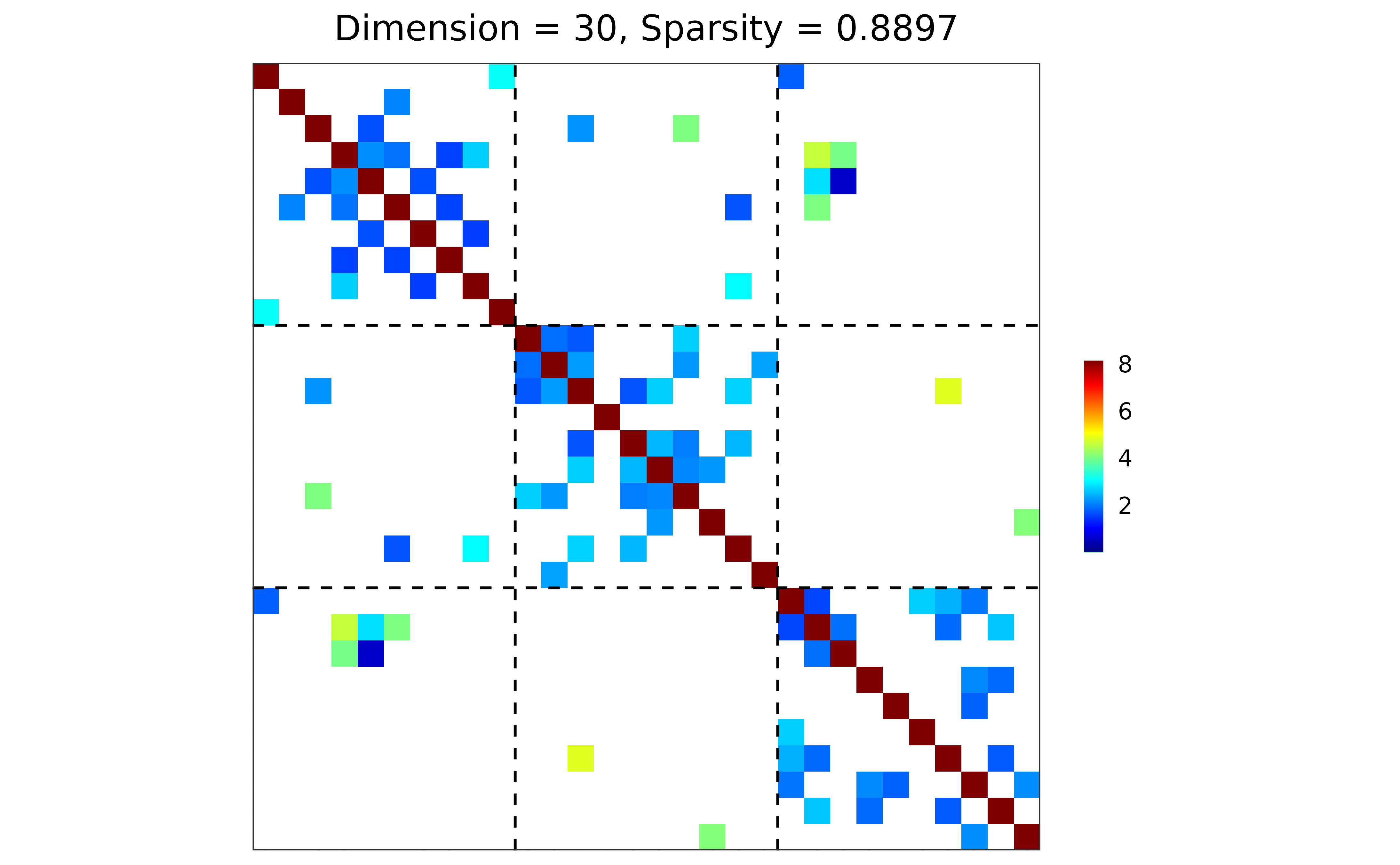
## block-structured precision matrix based on SBM
sim <- gen_prec_sbm(p = 30, K = 3,
within.prob = 0.25, between.prob = 0.05,
weight.dists = list("gamma", "unif"),
weight.paras = list(c(shape = 20, rate = 10),
c(min = 0, max = 5)),
cond.target = 100)
## ground truth visualization
plot(sim)
 ## n-by-p data matrix
library(MASS)
X <- mvrnorm(n = 20, mu = rep(0, 30), Sigma = sim$Sigma)
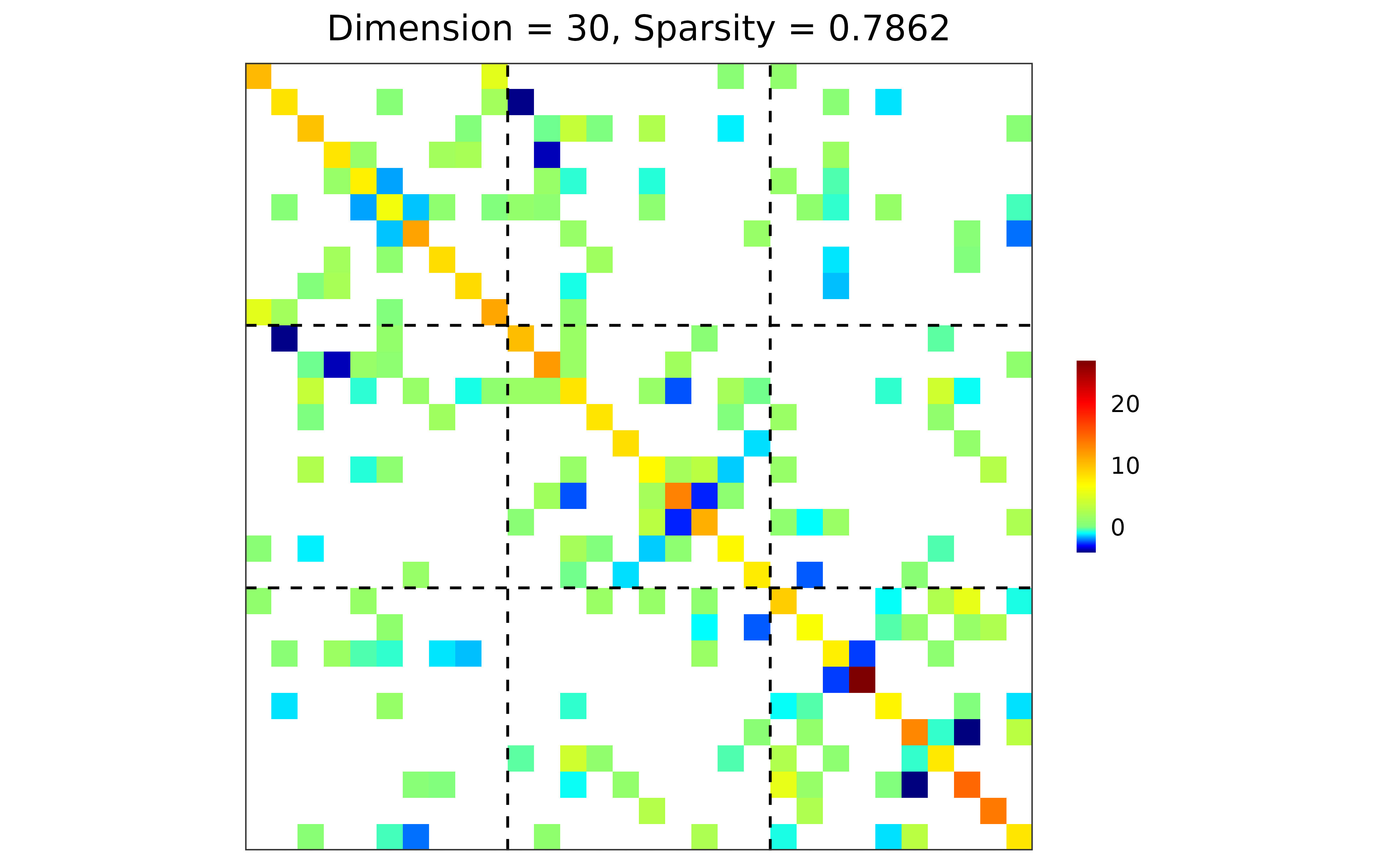
## precision matrix: adaptive lasso; BIC
prec <- grasps(X = X, membership = sim$membership, penalty = "adapt", crit = "BIC")
## precision matrix visualization
plot(prec)
## n-by-p data matrix
library(MASS)
X <- mvrnorm(n = 20, mu = rep(0, 30), Sigma = sim$Sigma)
## precision matrix: adaptive lasso; BIC
prec <- grasps(X = X, membership = sim$membership, penalty = "adapt", crit = "BIC")
## precision matrix visualization
plot(prec)
 ## performance
performance(hatOmega = prec$hatOmega, Omega = sim$Omega)
#> measure value
#> 1 sparsity 0.7862
#> 2 Frobenius 34.8430
#> 3 KL 12.5488
#> 4 quadratic 161.4326
#> 5 spectral 19.8343
#> 6 TP 24.0000
#> 7 TN 318.0000
#> 8 FP 69.0000
#> 9 FN 24.0000
#> 10 TPR 0.5000
#> 11 FPR 0.1783
#> 12 F1 0.3404
#> 13 MCC 0.2459
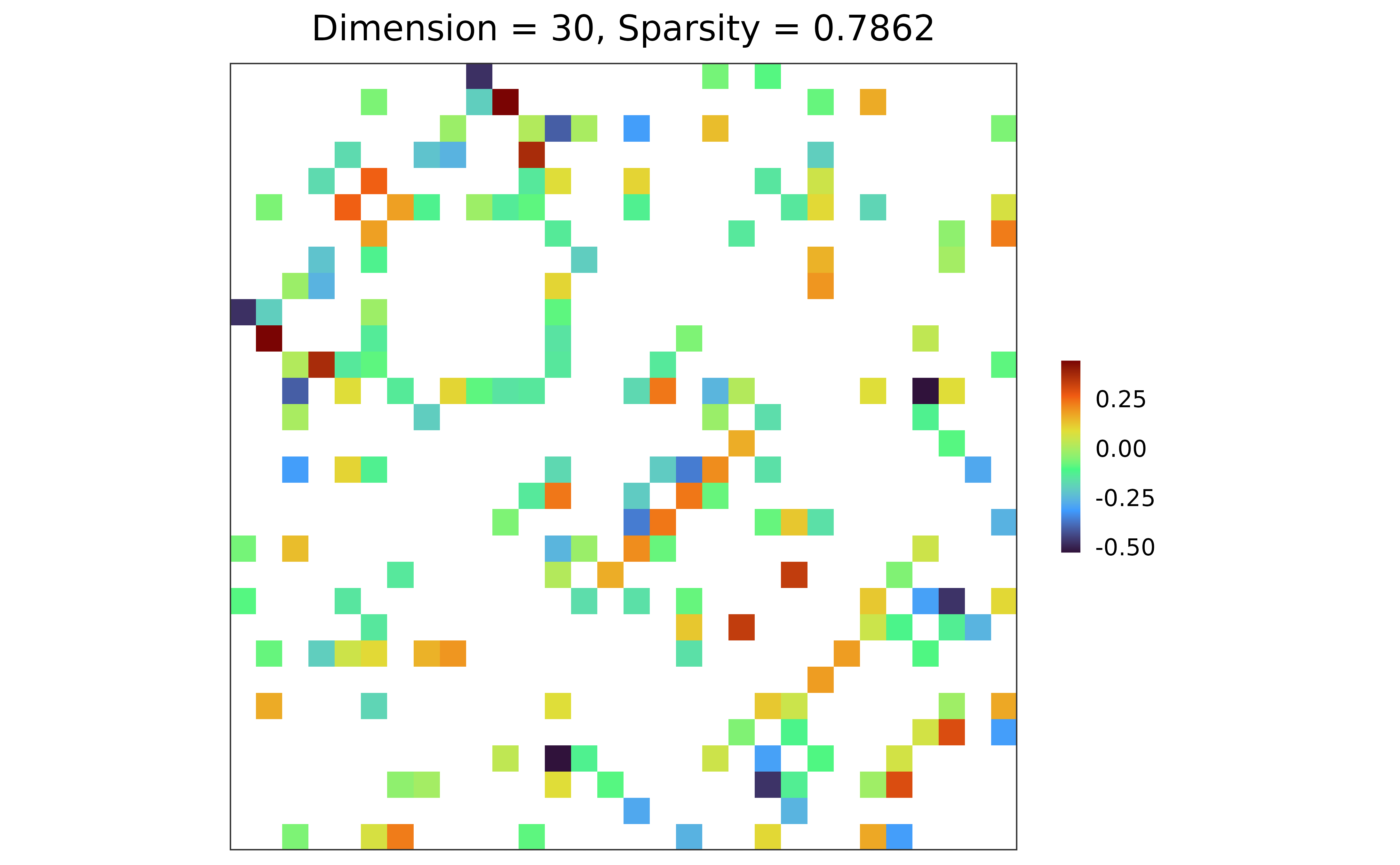
## adjacency matrix: diagonal = 0; raw partial correlations;
## no thresholding; weighted network
adj <- prec_to_adj(prec$hatOmega,
diag.zero = TRUE, absolute = FALSE,
threshold = NULL, weighted = TRUE)
## adjacency matrix visualization
plot(adj)
## performance
performance(hatOmega = prec$hatOmega, Omega = sim$Omega)
#> measure value
#> 1 sparsity 0.7862
#> 2 Frobenius 34.8430
#> 3 KL 12.5488
#> 4 quadratic 161.4326
#> 5 spectral 19.8343
#> 6 TP 24.0000
#> 7 TN 318.0000
#> 8 FP 69.0000
#> 9 FN 24.0000
#> 10 TPR 0.5000
#> 11 FPR 0.1783
#> 12 F1 0.3404
#> 13 MCC 0.2459
## adjacency matrix: diagonal = 0; raw partial correlations;
## no thresholding; weighted network
adj <- prec_to_adj(prec$hatOmega,
diag.zero = TRUE, absolute = FALSE,
threshold = NULL, weighted = TRUE)
## adjacency matrix visualization
plot(adj)