Introduction
Precision matrix estimation requires selecting appropriate regularization parameter \(\lambda\) to balance sparsity (number of edges) and model fit (likelihood), and a mixing parameter \(\alpha\) to trade off between element-wise (individual-level) and block-wise (group-level) penalties.
Background: Negative Log-Likelihood
In a Gaussian graphical model (GGM), the data matrix \(X_{n \times p}\) consists of \(n\) independent and identically distributed observations \(X_1, \dots, X_n\) drawn from \(N_p(\mu,\Sigma)\). Let \(\Omega = \Sigma^{-1}\) denote the precision matrix, and define the empirical covariance matrix as \(S = n^{-1} \sum_{i=1}^n (X_i-\bar{X})(X_i-\bar{X})^\top\). Up to an additive constant, the negative log-likelihood (nll) for \(\Omega\) simplified to \[ \mathrm{nll}(\Omega) = \frac{n}{2}[-\log\det(\Omega) + \mathrm{tr}(S\Omega)]. \] The edge set \(E(\Omega)\) is determined by the non-zero off-diagonal entries: an edge \((i, j)\) is included if and only if \(\omega_{ij} \neq 0\) for \(i < j\). The number of edges is therefore given by \(\vert E(\Omega) \vert\).
Selection Criteria
- AIC: Akaike information criterion (Akaike 1973)
\[ \hat{\Omega}_{\mathrm{AIC}} = {\arg\min}_{\Omega} \left\{ 2\,\mathrm{nll}(\Omega) + 2\,\lvert E(\Omega) \rvert \right\}. \]
- BIC: Bayesian information criterion (Schwarz 1978)
\[ \hat{\Omega}_{\mathrm{BIC}} = {\arg\min}_{\Omega} \left\{ 2\,\mathrm{nll}(\Omega) + \log(n)\,\lvert E(\Omega) \rvert \right\}. \]
- EBIC: Extended Bayesian information criterion (Chen and Chen 2008; Foygel and Drton 2010)
\[ \hat{\Omega}_{\mathrm{EBIC}} = {\arg\min}_{\Omega} \left\{ 2\,\mathrm{nll}(\Omega) + \log(n)\,\lvert E(\Omega) \rvert + 4\,\xi\,\log(p)\,\lvert E(\Omega) \rvert \right\}, \]
where \(\xi \in [0,1]\) is a tuning parameter. Setting \(\xi = 0\) reduces EBIC to the classic BIC.
- HBIC: High dimensional Bayesian information criterion (Wang et al. 2013; Fan et al. 2017)
\[ \hat{\Omega}_{\mathrm{HBIC}} = {\arg\min}_{\Omega} \left\{ 2\,\mathrm{nll}(\Omega) + \log[\log(n)]\,\log(p)\,\lvert E(\Omega) \rvert \right\}. \]
- \(K\)-fold cross validation with negative log-likelihood loss.
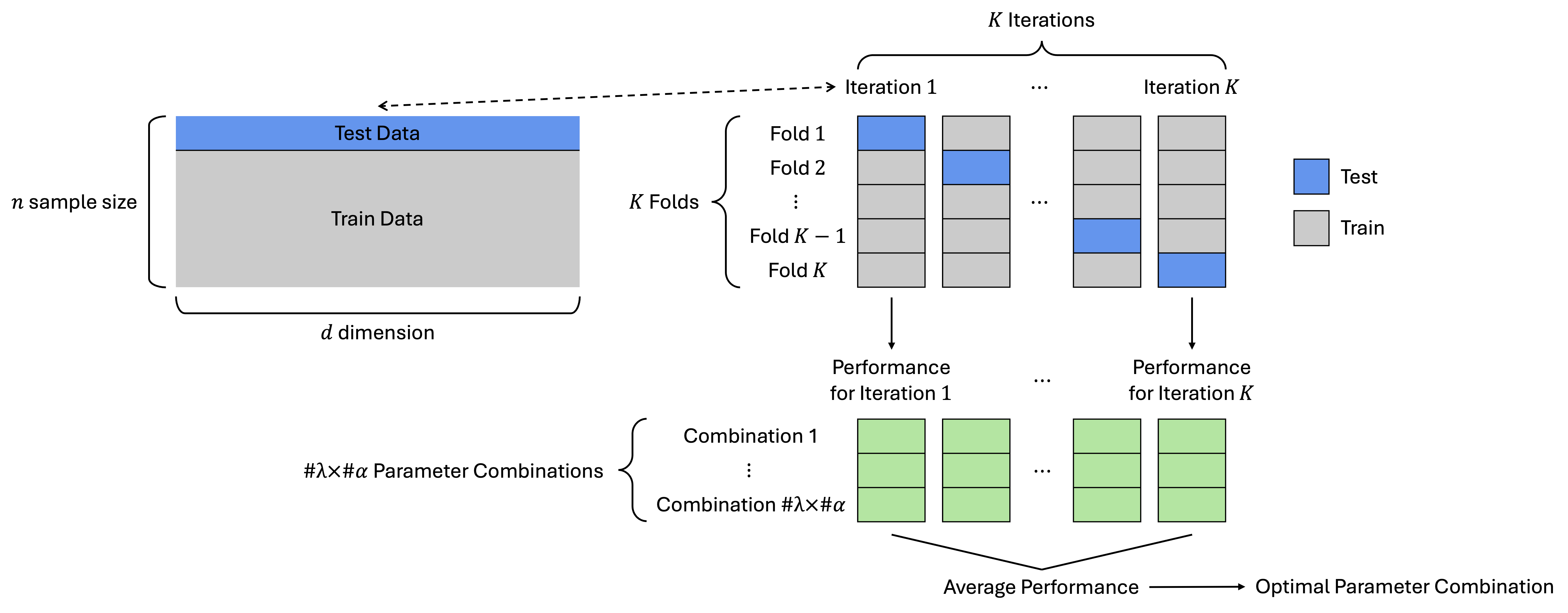
Figure 1 illustrates the \(K\)-fold cross-validation procedure used for tuning the parameters \(\lambda\) and \(\alpha\). The notation \(\#\lambda\) and \(\#\alpha\) denotes the number of candidate values considered for \(\lambda\) and \(\alpha\), respectively, forming a grid of \(\mathrm{\#}\lambda \times \mathrm{\#}\alpha\) total parameter combinations. For each of the \(K\) iterations, negative log-likelihood loss is evaluated for all parameter combinations, yielding \(K\) performance values per combination. The optimal parameter pair is selected as the one achieving the lowest average loss across the \(K\) iterations.