Convert a precision matrix to a partial-correlation-based adjacency matrix.
Usage
prec_to_adj(
  prec.mat,
  diag.zero = TRUE,
  absolute = FALSE,
  threshold = NULL,
  weighted = TRUE
)
Arguments
- prec.mat
A numeric precision matrix.
- diag.zero
A logical value (default = TRUE) specifying whether to set the diagonal entries of the adjacency matrix to 0. If
diag.zero = FALSE, the diagonal entries are set to 1 for a weighted network. For an unweighted network (weighted = FALSE), the diagonal is always forced to 0 to avoid self-loops.- absolute
A logical value (default = FALSE) specifying whether to take the absolute values of the partial correlations.
- threshold
A nonnegative numeric value (default =
NULL) specifying the threshold for edge filtering. Entries with absolute values smaller than the threshold are set to 0.- weighted
A logical value (default = TRUE) specifying whether to return a weighted adjacency matrix. If
weighted = FALSE, the matrix is a binary adjacency matrix with entries equal to 0 or 1.
Details
For a precision matrix \(\Omega\), the partial correlation between nodes \(i\) and \(j\) is computed as $$\rho_{ij} = - \frac{\Omega_{ij}}{\sqrt{\Omega_{ii}\Omega_{jj}}}.$$
Examples
library(grasps)
## reproducibility for everything
set.seed(1234)
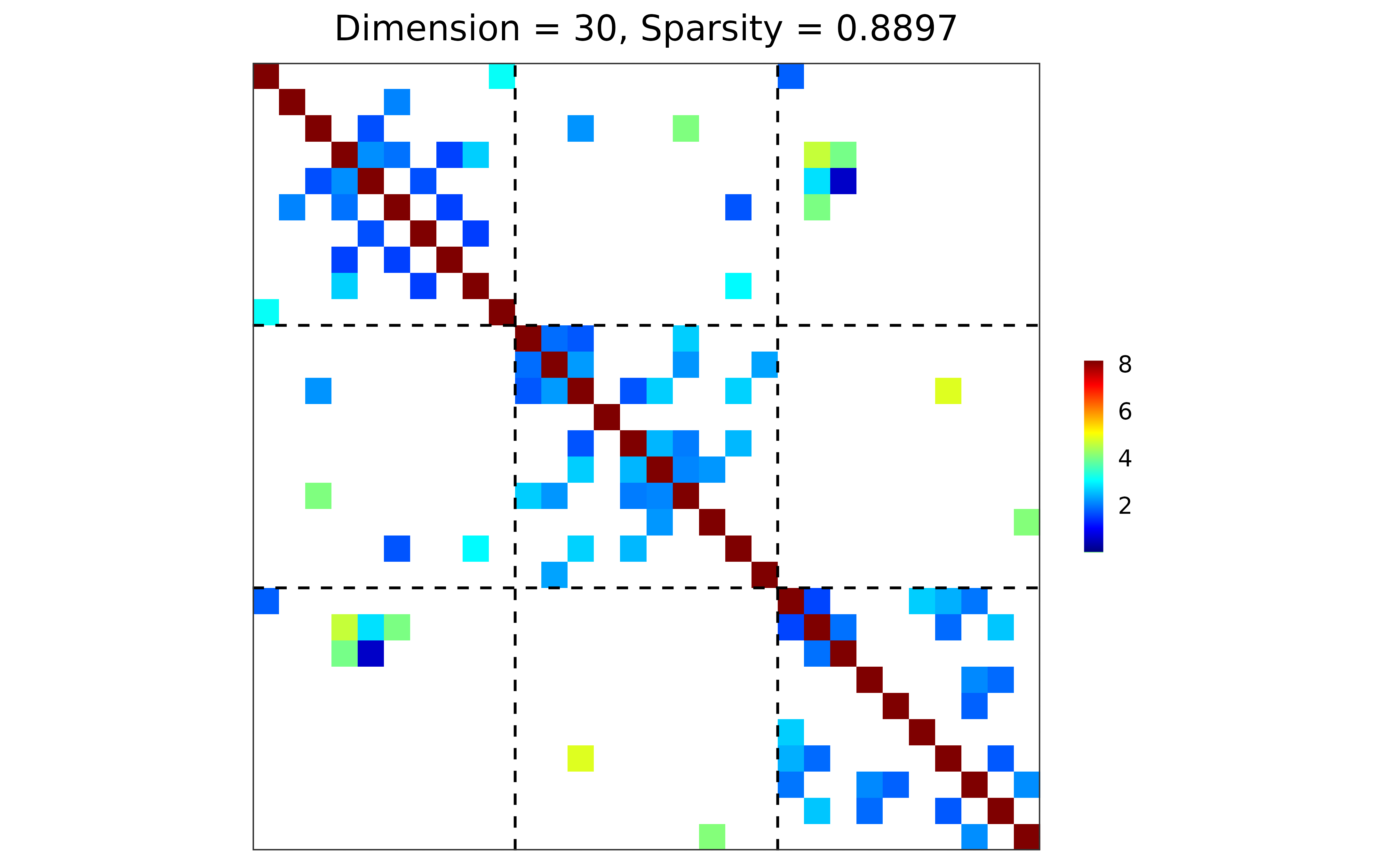
## block-structured precision matrix based on SBM
sim <- gen_prec_sbm(p = 30, K = 3,
within.prob = 0.25, between.prob = 0.05,
weight.dists = list("gamma", "unif"),
weight.paras = list(c(shape = 20, rate = 10),
c(min = 0, max = 5)),
cond.target = 100)
## ground truth visualization
plot(sim)
 ## n-by-p data matrix
library(MASS)
X <- mvrnorm(n = 20, mu = rep(0, 30), Sigma = sim$Sigma)
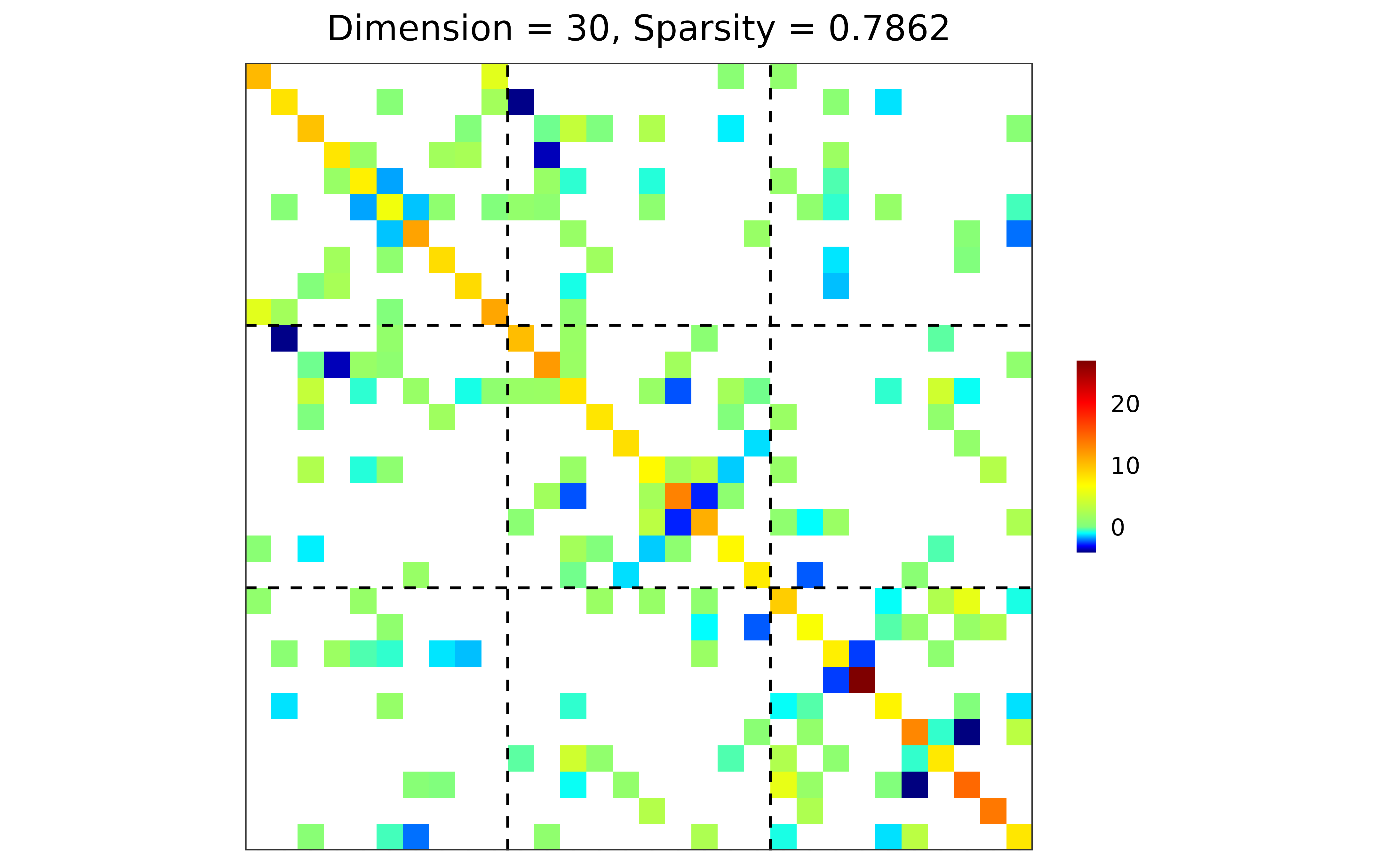
## precision matrix: adaptive lasso; BIC
prec <- grasps(X = X, membership = sim$membership, penalty = "adapt", crit = "BIC")
## precision matrix visualization
plot(prec)
## n-by-p data matrix
library(MASS)
X <- mvrnorm(n = 20, mu = rep(0, 30), Sigma = sim$Sigma)
## precision matrix: adaptive lasso; BIC
prec <- grasps(X = X, membership = sim$membership, penalty = "adapt", crit = "BIC")
## precision matrix visualization
plot(prec)
 ## performance
performance(hatOmega = prec$hatOmega, Omega = sim$Omega)
#> measure value
#> 1 sparsity 0.7862
#> 2 Frobenius 34.8430
#> 3 KL 12.5488
#> 4 quadratic 161.4326
#> 5 spectral 19.8343
#> 6 TP 24.0000
#> 7 TN 318.0000
#> 8 FP 69.0000
#> 9 FN 24.0000
#> 10 TPR 0.5000
#> 11 FPR 0.1783
#> 12 F1 0.3404
#> 13 MCC 0.2459
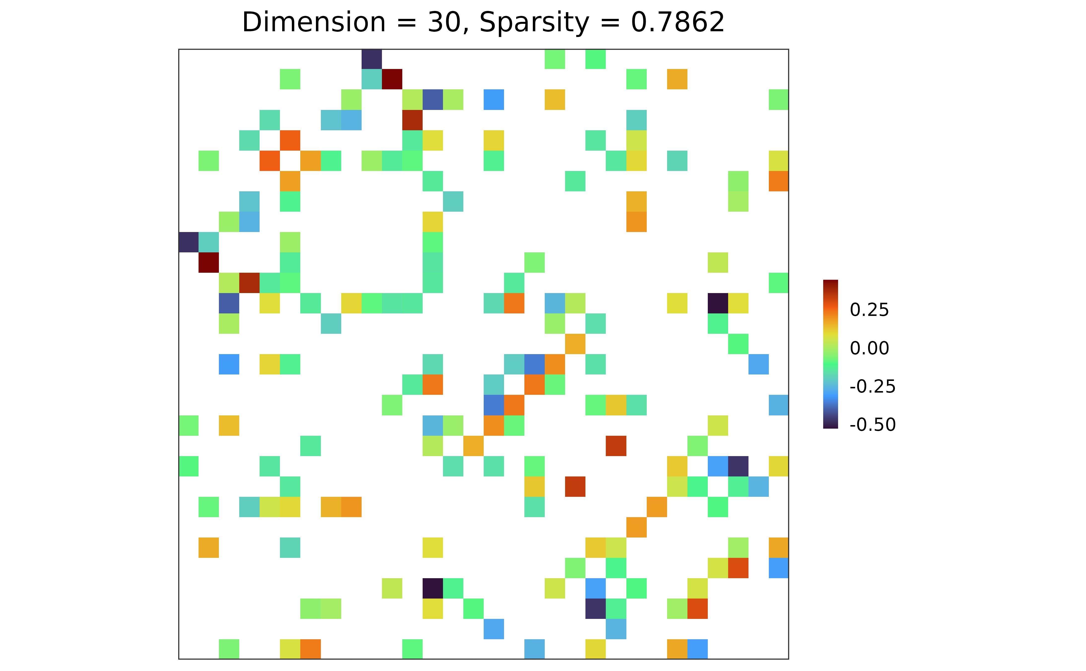
## adjacency matrix: diagonal = 0; raw partial correlations;
## no thresholding; weighted network
adj <- prec_to_adj(prec$hatOmega,
diag.zero = TRUE, absolute = FALSE,
threshold = NULL, weighted = TRUE)
## adjacency matrix visualization
plot(adj)
## performance
performance(hatOmega = prec$hatOmega, Omega = sim$Omega)
#> measure value
#> 1 sparsity 0.7862
#> 2 Frobenius 34.8430
#> 3 KL 12.5488
#> 4 quadratic 161.4326
#> 5 spectral 19.8343
#> 6 TP 24.0000
#> 7 TN 318.0000
#> 8 FP 69.0000
#> 9 FN 24.0000
#> 10 TPR 0.5000
#> 11 FPR 0.1783
#> 12 F1 0.3404
#> 13 MCC 0.2459
## adjacency matrix: diagonal = 0; raw partial correlations;
## no thresholding; weighted network
adj <- prec_to_adj(prec$hatOmega,
diag.zero = TRUE, absolute = FALSE,
threshold = NULL, weighted = TRUE)
## adjacency matrix visualization
plot(adj)