Plot Function for S3 Class "penderiv"

Generate a visualization of penalty functions produced by compute_penalty, or penalty derivatives produced by compute_derivative. The plot automatically summarizes multiple configurations of penalty type, \(\lambda\), and \(\gamma\). Optional zooming is supported through facet_zoom.

Usage

# S3 method for class 'penderiv'
plot(x, ...)

Arguments

x

An object inheriting from S3 class "penderiv", typically returned by compute_penalty, or compute_derivative.

...

Optional arguments passed to facet_zoom to zoom in on a subset of the data, while keeping the view of the full dataset as a separate panel.

Value

An object of class ggplot.

Examples

library(grasps)
library(ggplot2)

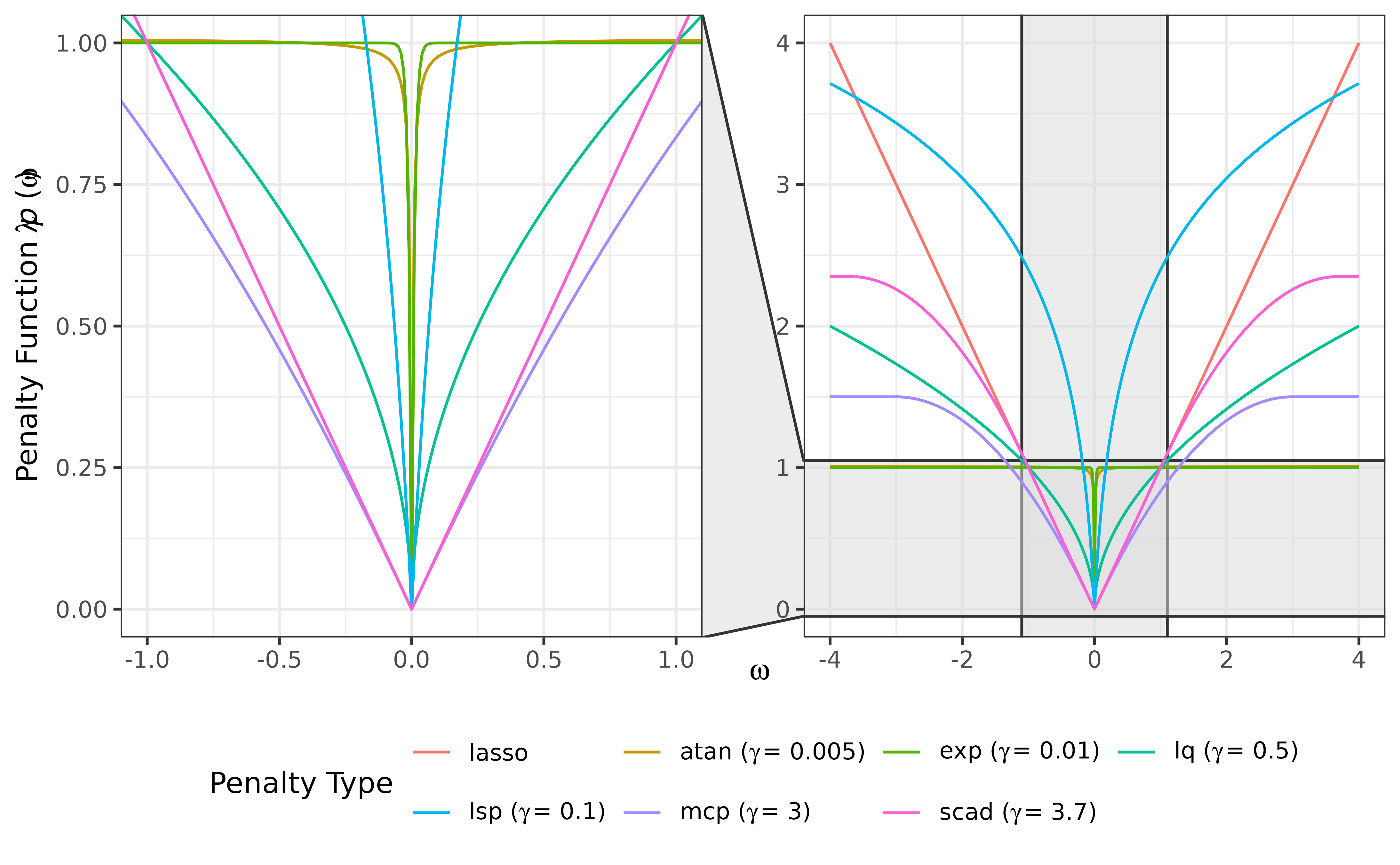
pen_df <- compute_penalty(
  omega = seq(-4, 4, by = 0.01),
  penalty = c("atan", "exp", "lasso", "lq", "lsp", "mcp", "scad"),
  lambda = 1)

plot(pen_df, xlim = c(-1, 1), ylim = c(0, 1), zoom.size = 1) +
  guides(color = guide_legend(nrow = 2, byrow = TRUE))


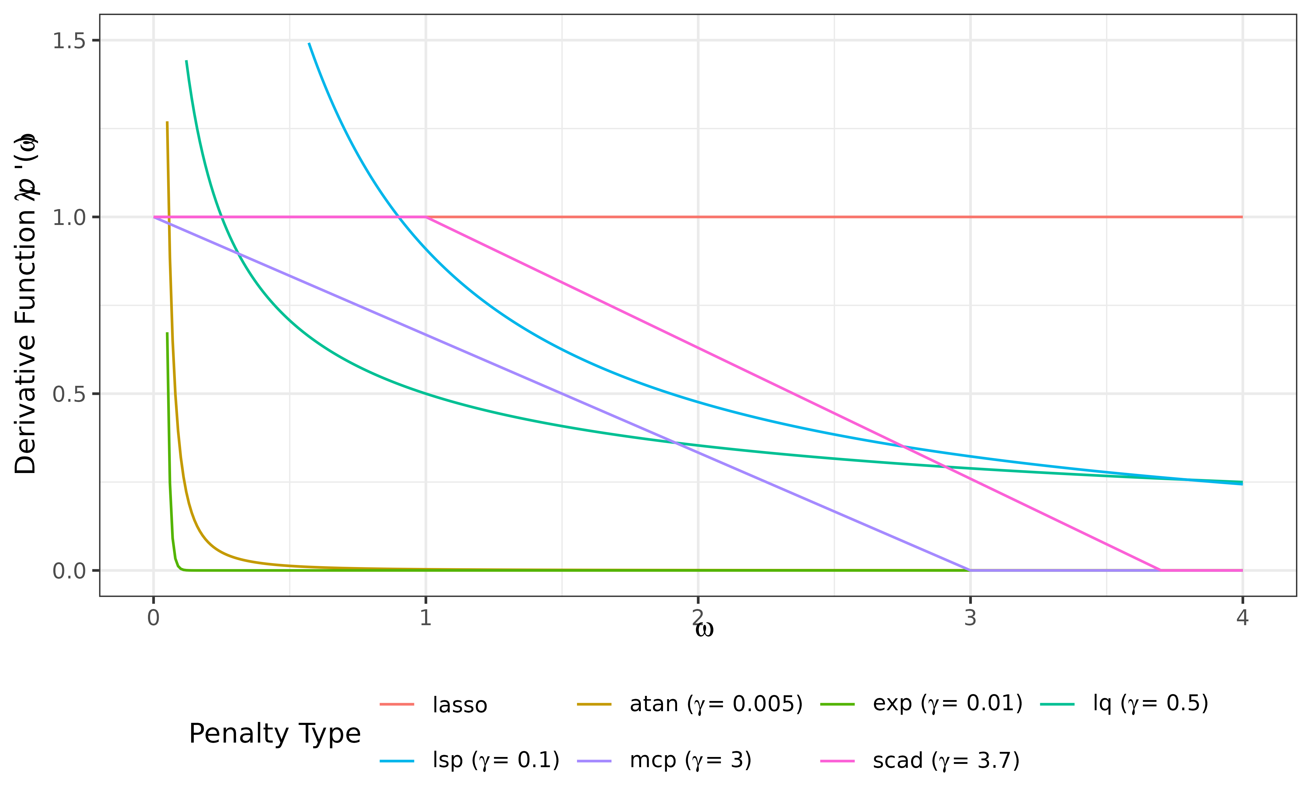
deriv_df <- compute_derivative(
  omega = seq(0, 4, by = 0.01),
  penalty = c("atan", "exp", "lasso", "lq", "lsp", "mcp", "scad"),
  lambda = 1)

plot(deriv_df) +
  scale_y_continuous(limits = c(0, 1.5)) +
  guides(color = guide_legend(nrow = 2, byrow = TRUE))
#> Warning: Removed 79 rows containing missing values or values outside the scale range
#> (`geom_line()`).