library(grasps) ## for penalty computation
library(ggplot2) ## for visualization

penalties <- c("atan", "exp", "lasso", "lq", "lsp", "mcp", "scad")

pen_df <- compute_penalty(seq(-4, 4, by = 0.01), penalties, lambda = 1)
plot(pen_df, xlim = c(-1, 1), ylim = c(0, 1), zoom.size = 1) +
guides(color = guide_legend(nrow = 2, byrow = TRUE))Preliminary
Consider the following setting:
Gaussian graphical model (GGM) assumption:
The data \(X_{p \times p}\) consists of independent and identically distributed samples \(X_1, \dots, X_n \sim N_p(\mu,\Sigma)\).Disjoint group structure:
The \(p\) variables can be partitioned into disjoint groups.Goal:
Estimate the precision matrix \(\Omega = \Sigma^{-1} = (\omega_{ij})_{p \times p}\).
Sparse-Group Estimator
\[\begin{gather} \hat{\Omega}(\lambda,\alpha,\gamma) = {\arg\min}_{\Omega \succ 0} \left\{ -\log\det(\Omega) + \text{tr}(S\Omega) + \mathcal{P}_{\lambda,\alpha,\gamma}(\Omega) \right\}, \\[10pt] \mathcal{P}_{\lambda,\alpha,\gamma}(\Omega) = \alpha \mathcal{P}^\text{idv}_{\lambda,\gamma}(\Omega) + (1-\alpha) \mathcal{P}^\text{grp}_{\lambda,\gamma}(\Omega), \\[10pt] \mathcal{P}^\text{idv}_{\lambda,\gamma}(\Omega) = \sum_{i,j} P_{\lambda,\gamma}(\lvert\omega_{ij}\rvert), \\[5pt] \mathcal{P}^\text{grp}_{\lambda,\gamma}(\Omega) = \sum_{g,g^\prime} P_{\lambda,\gamma}(\lVert\Omega_{gg^\prime}\rVert_F). \end{gather}\]
where:
\(S = n^{-1} \sum_{i=1}^n (X_i-\bar{X})(X_i-\bar{X})^\top\) is the empirical covariance matrix.
\(\lambda \geq 0\) is the global regularization parameter controlling overall shrinkage.
\(\alpha \in [0,1]\) is the mixing parameter controlling the balance between element-wise and block-wise penalties.
\(\gamma\) is the additional parameter for non-convex penalties, controlling the degree of nonconvexity (or concavity) of the penalty function.
\(\mathcal{P}_{\lambda,\alpha,\gamma}(\Omega)\) is a generic bi-level penalty template that combines element-wise and block-wise regularization, allowing convex or non-convex regularizers while preserving the intrinsic group structure among variables.
\(\mathcal{P}^\text{idv}_{\lambda,\gamma}(\Omega)\) is the element-wise individual penalty component.
\(\mathcal{P}^\text{grp}_{\lambda,\gamma}(\Omega)\) is the block-wise group penalty component.
\(P_{\lambda,\gamma}(\cdot)\) is the penalty function.
\(\Omega_{gg^\prime}\) is the submatrix of \(\Omega\) with the rows from group \(g\) and columns from group \(g^\prime\).
The Frobenius norm \(\lVert\Omega\rVert_F\) is defined as \(\lVert\Omega\rVert_F = (\sum_{i,j} \lvert\omega_{ij}\rvert^2)^{1/2} = [\text{tr}(\Omega^\top\Omega)]^{1/2}\).
Note:
- The parameter \(\gamma\) is only relevant for non-convex penalties. The Lasso penalty can be viewed as a special case in which \(\gamma\) is not required.
Penalties
- Lasso: Least absolute shrinkage and selection operator (Tibshirani 1996; Friedman et al. 2008)
\[P_\lambda(\omega_{ij}) = \lambda\vert\omega_{ij}\vert.\]
- Adaptive lasso (Zou 2006; Fan et al. 2009)
\[
P_{\lambda,\gamma}(\omega_{ij}) = \lambda\frac{\vert\omega_{ij}\vert}{v_{ij}},
\] where \(V = (v_{ij})_{d \times d} = (\vert\tilde{\omega}_{ij}\vert^\gamma)_{d \times d}\) is a matrix of adaptive weights, and \(\tilde{\omega}_{ij}\) is the initial estimate obtained using penalty = "lasso".
- Atan: Arctangent type penalty (Wang and Zhu 2016)
\[ P_{\lambda,\gamma}(\omega_{ij}) = \lambda(\gamma+\frac{2}{\pi}) \arctan\left(\frac{\vert\omega_{ij}\vert}{\gamma}\right), \quad \gamma > 0. \]
- Exp: Exponential type penalty (Wang et al. 2018)
\[ P_{\lambda,\gamma}(\omega_{ij}) = \lambda\left[1-\exp\left(-\frac{\vert\omega_{ij}\vert}{\gamma}\right)\right], \quad \gamma > 0. \]
\[ P_{\lambda,\gamma}(\omega_{ij}) = \lambda\vert\omega_{ij}\vert^\gamma, \quad 0 < \gamma < 1. \]
- LSP: Log-sum penalty (Candès et al. 2008)
\[ P_{\lambda,\gamma}(\omega_{ij}) = \lambda\log\left(1+\frac{\vert\omega_{ij}\vert}{\gamma}\right), \quad \gamma > 0. \]
- MCP: Minimax concave penalty (Zhang 2010)
\[ P_{\lambda,\gamma}(\omega_{ij}) = \begin{cases} \lambda\vert\omega_{ij}\vert - \dfrac{\omega_{ij}^2}{2\gamma}, & \text{if } \vert\omega_{ij}\vert \leq \gamma\lambda, \\ \dfrac{1}{2}\gamma\lambda^2, & \text{if } \vert\omega_{ij}\vert > \gamma\lambda. \end{cases} \quad \gamma > 1. \]
- SCAD: Smoothly clipped absolute deviation (Fan and Li 2001; Fan et al. 2009)
\[ P_{\lambda,\gamma}(\omega_{ij}) = \begin{cases} \lambda\vert\omega_{ij}\vert & \text{if } \vert\omega_{ij}\vert \leq \lambda, \\ \dfrac{2\gamma\lambda\vert\omega_{ij}\vert-\omega_{ij}^2-\lambda^2}{2(\gamma-1)} & \text{if } \lambda < \vert\omega_{ij}\vert < \gamma\lambda, \\ \dfrac{\lambda^2(\gamma+1)}{2} & \text{if } \vert\omega_{ij}\vert \geq \gamma\lambda. \end{cases} \quad \gamma > 2. \]
Note:
- For Lasso, which is convex, the additional parameter \(\gamma\) is not required, and the penalty function \(P_{\lambda,\gamma}(\cdot)\) simplifies to \(P_\lambda(\cdot)\).
Illustrative Visualization
Figure 1 illustrates a comparison of various penalty functions \(P(\omega)\) evaluated over a range of \(\omega\) values. The main panel (right) provides a wider view of the penalty functions’ behavior for larger \(\vert\omega\vert\), while the inset panel (left) magnifies the region near zero \([-1, 1]\).
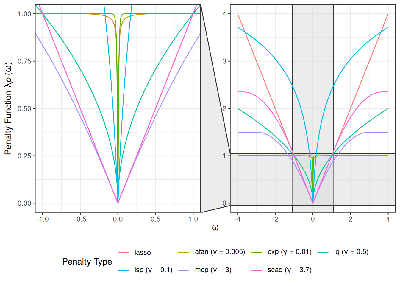
Figure 2 displays the derivative function \(P^\prime(\omega)\) associated with a range of penalty types. The Lasso exhibits a constant derivative, corresponding to uniform shrinkage. For MCP and SCAD, the derivatives are piecewise: initially equal to the Lasso derivative, then decreasing over an intermediate region, and eventually dropping to zero, indicating that large \(\vert\omega\vert\) receive no shrinkage. Other non-convex penalties show smoothly diminishing derivatives as \(\vert\omega\vert\) increases, reflecting their tendency to shrink small \(\vert\omega\vert\) strongly while exerting little to no shrinkage on large ones.
deriv_df <- compute_derivative(seq(0, 4, by = 0.01), penalties, lambda = 1)
plot(deriv_df) +
  scale_y_continuous(limits = c(0, 1.5)) +
  guides(color = guide_legend(nrow = 2, byrow = TRUE))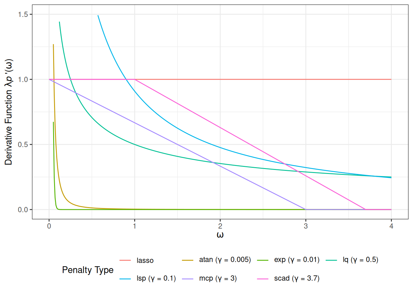
Reference
Candès, Emmanuel J., Michael B. Wakin, and Stephen P. Boyd. 2008. “Enhancing Sparsity by Reweighted \(\ell_1\) Minimization.” Journal of Fourier Analysis and Applications 14 (5): 877–905. https://doi.org/10.1007/s00041-008-9045-x.
Fan, Jianqing, Yang Feng, and Yichao Wu. 2009. “Network Exploration via the Adaptive LASSO and SCAD Penalties.” The Annals of Applied Statistics 3 (2): 521–41. https://doi.org/10.1214/08-aoas215.
Fan, Jianqing, and Runze Li. 2001. “Variable Selection via Nonconcave Penalized Likelihood and Its Oracle Properties.” Journal of the American Statistical Association 96 (456): 1348–60. https://doi.org/10.1198/016214501753382273.
Frank, Lldiko E., and Jerome H. Friedman. 1993. “A Statistical View of Some Chemometrics Regression Tools.” Technometrics 35 (2): 109–35. https://doi.org/10.1080/00401706.1993.10485033.
Friedman, Jerome, Trevor Hastie, and Robert Tibshirani. 2008. “Sparse Inverse Covariance Estimation with the Graphical Lasso.” Biostatistics 9 (3): 432–41. https://doi.org/10.1093/biostatistics/kxm045.
Fu, Wenjiang J. 1998. “Penalized Regressions: The Bridge Versus the Lasso.” Journal of Computational and Graphical Statistics 7 (3): 397–416. https://doi.org/10.1080/10618600.1998.10474784.
Tibshirani, Robert. 1996. “Regression Shrinkage and Selection via the Lasso.” Journal of the Royal Statistical Society: Series B (Methodological) 58 (1): 267–88. https://doi.org/10.1111/j.2517-6161.1996.tb02080.x.
Wang, Yanxin, Qibin Fan, and Li Zhu. 2018. “Variable Selection and Estimation Using a Continuous Approximation to the \(L_0\) Penalty.” Annals of the Institute of Statistical Mathematics 70 (1): 191–214. https://doi.org/10.1007/s10463-016-0588-3.
Wang, Yanxin, and Li Zhu. 2016. “Variable Selection and Parameter Estimation with the Atan Regularization Method.” Journal of Probability and Statistics 2016: 6495417. https://doi.org/10.1155/2016/6495417.
Zhang, Cun-Hui. 2010. “Nearly Unbiased Variable Selection Under Minimax Concave Penalty.” The Annals of Statistics 38 (2): 894–942. https://doi.org/10.1214/09-AOS729.
Zou, Hui. 2006. “The Adaptive Lasso and Its Oracle Properties.” Journal of the American Statistical Association 101 (476): 1418–29. https://doi.org/10.1198/016214506000000735.